Introduction
On this little project of making a guitar effect chain, the equalizer/filter will be a central component. The guitar has a particular spectrum, and not everything within the 20KHz humans can hear needs to be processed. In filtering out the unnecessary frequencies we get some benefits:
- All the spectral content is useful information, increasing the amount of signal we can process
- We are cutting noise, which is usually very wideband, often modeled as uniformly distributed
All of this translates into a better signal-to-noise ratio (SNR).
That’s not the only benefit we get from a filter, though, as we can also use it to shape the spectrum of the sound, boosting or attenuating certain bands as we want. For this implementation I chose a finite impulse response (FIR) filter. This is quite easy to implement in an FPGA in principle, since it’s just a buffer of samples in some kind of FIFO, a memory to store the correcting taps, some multipliers, and a final summation of all the calculated values. It would look something like this:
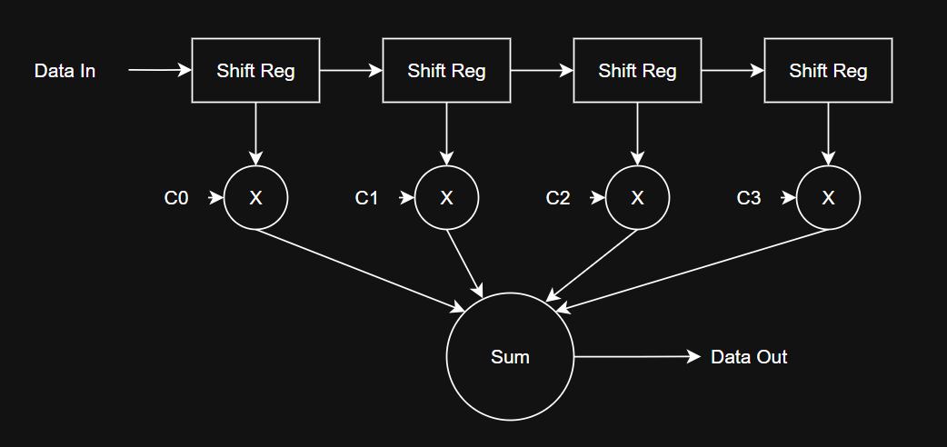
Example of FIR implementation with 4 taps
In the picture there is a 4-tap FIR filter: it needs 4 coefficients previously calculated and stored in some memory, some shift registers, and a final sum. As you can see, it’s quite a simple circuit that follows simple mathematics. With its simplicity comes great flexibility in how to implement it, and this is what we will be discussing here.
Design Tradeoff
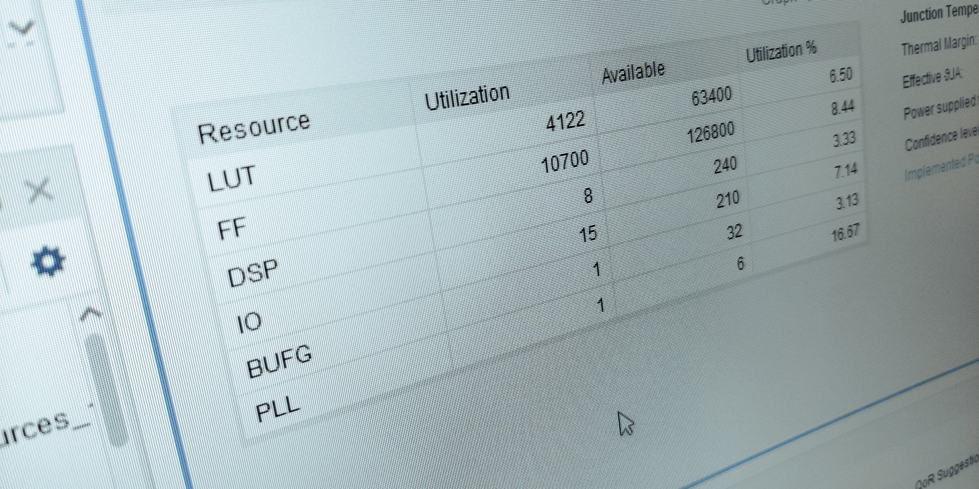
On first approximation, the granularity of the frequency response — that is, how good this filter is at manipulating narrow bands — depends on the number of taps. However, on my board I have DSP cells that implement multiplication, not too many mind you, 240 in my case. This means that, at 48KHz, if I blindly used all the DSP cells to implement the filter, I could manipulate bands as narrow as 200Hz — not bad, if it weren’t for the fact that I’d be left without hardware for anything else. So, let’s make some considerations here:
- The Arty operates in the megahertz range, but I need to process data at 48KHz
- I can afford some audible delay, on the order of 10ms at most
Hence, what I’ll do is use only 8 DSP cells that run through the FIFO and the tap memory, multiplying and accumulating (a feature of the Artix DSP cells) the results. This has the additional advantage of reducing the complexity of the final adder for large tap counts. This operation happens at 60MHz, so if we wanted 256 taps, with 8 DSP cells we’d have to run through 32 data samples — taking around 2 microseconds. We have a budget of 20 microseconds from a sampling rate of 48KHz, so we’re good up to a few hundred FIR coefficients. This technique is called time-multiplexing.
FIR Design
As mentioned before, we need a way to store many samples for the calculation, so a basic shift register is implemented here.
| |
Then, a Finite State Machine (FSM) will be used to control the flow of the computation. Every time we get a new sample from the previous steps (at 48KHz), we start the machine to calculate the FIR value. When it’s done calculating, it’s set to IDLE and awaits the next sample. Fairly simple.
In doing those operations, we defined PARALLELISM, which is the number of DSP cells we want to use for the FIR implementation, and NUM_TAPS, which is the number of FIR coefficients. The FSM will run until NUM_MAC_STEPS calculations have been performed.
| |
Here we generate two variables: tap_idx, which is basically the address of the coefficient in memory, and mac_step, which keeps track of the parallel operation to conclude the FSM’s MAC state. With tap_idx we can select the taps to be used in the current multiplication step from the memory taps_flat. For the DSP cells, we also have to extend the data to 18-bit signed. We do this on a per-sample basis to avoid extra storage of extended data.
| |
And then the last step, where the magic happens. On a new sample, the accumulator and partial sum get reset. Then, in the MAC state, the multiplications happen. Here, it’s important to tell Vivado that we’ll be using DSP cells for multiplication with (* use_dsp = "yes" *), else it will try to use LUTs to synthesize them, which is expensive in hardware and fairly inefficient.
Also, for my specific use case, I unrolled the sum depending on how many DSP cells I want to use. I will mainly stick with 8, but one never knows.
| |
At every MAC_STEP we accumulate the partial_sum, and in the DONE state we propagate the result to the output to avoid glitches, also informing the next cell that the sample is ready.
Conclusion
Here we presented a digital implementation of a filter, where we trade off area/power consumption against delay. Since we can afford some delay, this tradeoff has overall benefits for the implementation without any extra complexity for the users of this block. For my use I will stick to 256/512 taps and 8 DSP units in parallel, still giving me the feel of real-time processing, no matter how hard I try to hear any kind of delay. In the next article I will be delving a bit into the analog part of this project, as I need a front end for the ADC.
Stay tuned.